Minimum KL $\rightarrow$ Maximum Likelihood

In this chapter, we'll explore what happens when we minimize the KL divergence between two distributions. Specifically, we'll look at the following problem that often comes up in statistics and machine learning:

We will solve this problem by taking $q \in Q$ that minimizes $D(p, q)$. If you remember the previous chapters, this should make plenty of sense! We will also see how a special case of this approach is equivalent to the maximum likelihood principle (MLE) in statistics.

Let's dive into the details!

Example: Gaussian fit

Here's the example I want you to have in mind. Imagine we have some data—for instance, the 16 foot length measurements $X_1, \dots, X_{16}$ from our statistics riddle. Assuming the order of the data points doesn't matter, it's convenient to represent them as an empirical distribution $p$, where each outcome is assigned a probability of $1/16$. This is what we call an empirical distribution. In some sense, this empirical distribution is the "best fit" for our data; it's the most precise distribution matching what we have observed.

However, this is a terrible predictive model—it assigns zero probability to outcomes not present in the data! If we were to measure the 17th person's foot, then unless we get one of the 16 lengths we've already seen, our model is going to be "infinitely surprised" by the new outcome, since it assigns zero probability for it.¹ We need a better model.

One common approach is to first identify a family of distributions $Q$ that we believe would be a good model for the data. Here, we might suspect that foot lengths follow a Gaussian distribution $N(\mu, \sigma^2)$.² In this case, $Q$ would be the set of all Gaussian distributions with varying means and variances.

In the following widget, you can see the KL divergence & cross-entropy between the empirical distribution $p_{empirical}$ and the model $q$.

In the widget, we computed KL divergence like this:

This is a bit fishy, since the formula combines probabilities for $p$ with probability densities for $q$. Fortunately, we don't need to worry about this too much. The only weird consequence of this is that the resulting numbers are sometimes smaller than zero which we've seen can't happen if we just plug in probabilities to both. ³

Remember: I.e., KL is the difference of cross-entropy and entropy. As , you can check that the two numbers in the widget above are always the same, up to a shift by 4.

I want to persuade you that if we are pressed against the wall and have to come up with the best Gaussian fitting the data, we should choose the Gaussian with $\mu, \sigma$ minimizing . Before arguing why this is sensible, I want to explain what this means in our scenario.

We can compute the best $\mu, \sigma$ by minimizing the right-hand side of [Eq. gauss-KL?]. This looks daunting, but in this case it's not too bad. We can rewrite it like this:

To find the best $\mu$, you can notice that whatever $\sigma$, finding the $\mu$ minimizing the right-hand side boils down to minimizing the expression $\sum_{i = 1}^{16} (x_i - \mu)^2$. It turns out this is minimized by $\mu_{best} = \frac{1}{16} \cdot \sum_{i = 1}^{16} x_i$. This formula is called the sample mean.

It may seem a bit underwhelming that we did all of this math just to compute the average of 16 numbers, but in a minute, we will see more interesting examples. We'll also revisit this problem in a later chapter and compute the formula for $\sigma$.

Why KL?

I claim that minimizing KL to find a model $q$ of data $p$ is a pretty good approach in general. Why?

Recall that KL divergence is designed to measure how well a model $q$ approximates the true distribution $p$. More specifically, it is the rate of how quickly a Bayesian detective learns that the true distribution is $p$, not $q$. So, minimizing KL simply means selecting the best "imposter" that it takes the longest to separate from the truth. That's pretty reasonable to me!

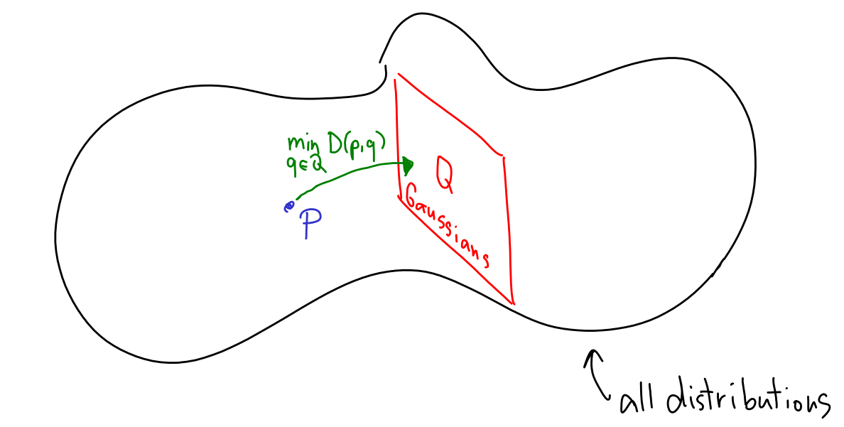
Visually, I like to think of it like this. First, imagine a "potato" of all possible distributions. The empirical distribution $p$ is a single lonely point within it. Then, there's a subset of distributions $Q$ that we believe would be a good model for the data. Although KL divergence is not, technically speaking, a distance between distributions, because it's asymmetric, it's close enough to think of it as a distance. Minimizing KL is then like finding the closest point in $Q$ to $p$; or, if you want, it's like projecting $p$ onto $Q$.

Cross-entropy loss

Let's write down our minimization formula, in its full glory:

Here, $x$ ranges over all possible values in the distribution. In our Gaussian example, we have seen how the KL divergence is actually tracking the cross-entropy. That's because their difference is simply the entropy of the original distribution $p$, and whatever it is, it stays the same for different models $q$ that we may try out.

This of course holds in general, which is why we can write:

In machine learning, we typically say that we find models of data by minimizing the cross-entropy. This is equivalent to minimizing KL divergence. It's good to know both -- Cross-entropy has a bit simpler formula, but KL divergence is a bit more fundamental which sometimes helps.⁴

Now, let's solve two of our riddles by minimizing the KL divergence / cross-entropy. First, we return to our Intelligence test riddle and see how neural networks are trained.

Let's also see how we can use cross-entropy score to grade experts from our prediction riddle.

Maximum likelihood principle

We already understand that there's not much difference between minimizing cross-entropy or KL divergence between $p$ and $q$, whenever $p$ is fixed. There's one more equivalent way to think about this. Let's write the cross-entropy formula once more:

In many scenarios, $p$ is literally just the uniform, empirical distribution over some data points $x_1, \dots, x_n$. In those cases, we can just write:

Another way to write this is:

The expressions like $q(x_i)$ (probability a data point $x_i$ has been generated from a probabilistic model $q \in Q$) are typically called likelihoods. The product $\prod_{i = 1}^n q(x_i)$ is the overall likelihood - it's the overall probability that the dataset $x_1, \dots, x_n$ was generated by the model $q$. So, minimizing the cross-entropy with $q$ is equivalent to maximizing the likelihood of $q$.

The methodology of selecting $q$ that maximizes $\prod_{i = 1}^n q(x_i)$ is called the maximum likelihood principle and it's considered one of the most important cornerstones of statistics. We can now see that it's pretty much the same as our methodology of minimizing KL divergence (which is in fact a bit more general as it works also for non-uniform $p$).

In a sense, this is not surprising at all. Let's remember how we defined KL divergence in the first chapter. It was all about the Bayesian detective trying to distinguish the truth from the imposter. But look—the detective accumulates evidence literally by multiplying her current probability distribution by the likelihoods. KL divergence / cross-entropy / entropy is just a useful language to talk about the accumulated evidence, since it's often easier to talk about "summing stuff" instead of "multiplying stuff".

So, the fact that minimizing cross-entropy is equivalent to maximizing the overall likelihood really just comes down to how we change our beliefs using Bayes' rule.

In the context of statistics, it's more common to talk about maximum likelihood principle (and instead of cross-entropy, you may hear about the log-likelihood). In the context of machine learning, it's more common to talk about cross-entropy / KL divergence (and instead of likelihoods, you may hear about perplexity).

There's a single versatile principle that underlies all the examples. Algebraically, we can think of it as: If you have to choose a model for $p$, try $q$ with the smallest $D(p,q)$. But ultimately, it's more useful if you can, in your head, compile this principle down to Bayes' rule: A good model is hard to distinguish from the truth by a Bayesian detective. ⁵

What's next?

In the next chapter, we will see what happens if we minimize the first parameter in $D(p, q)$.