Minimum KL $\rightarrow$ Maximum entropy

In the previous chapter, we saw what happens when we minimize $q$ in the KL divergence $D(p, q)$. We used this to find the best model of data $p$.

In this chapter, we will ponder the second question - what happens if we minimize $p$ in $D(p, q)$? This way, we will build the so-called maximum entropy principle that guides us whenever we want to choose a good model distribution.

Conditioning on steroids

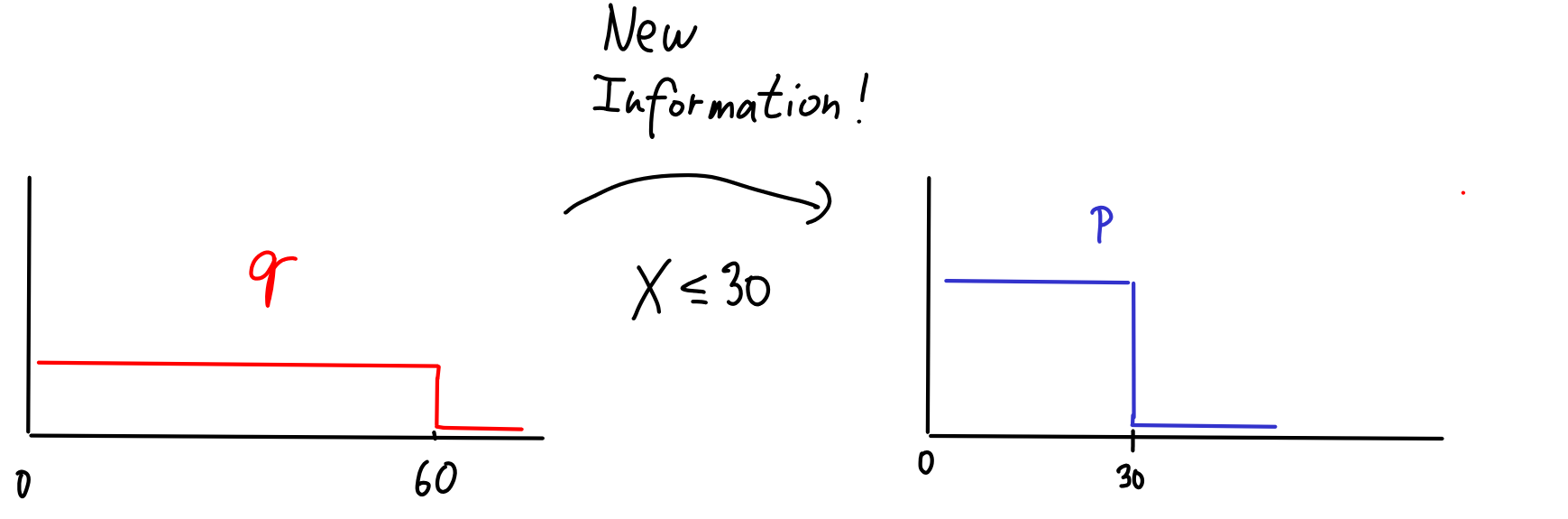
Suppose I want to determine a probability distribution modelling the random variable $X$ of how long it takes me to eat lunch. My initial (and very crude) model of $X$ might be a uniform distribution $q$ between and minutes.

Starting with this model, I can try to get some new information and condition on it to get a better model $p$.

For example, let's say that after eating many lunches, I observe that I always finish after at most 30 minutes. I can turn this into new information that $X \le 30$. I can condition on this information and get a better model:

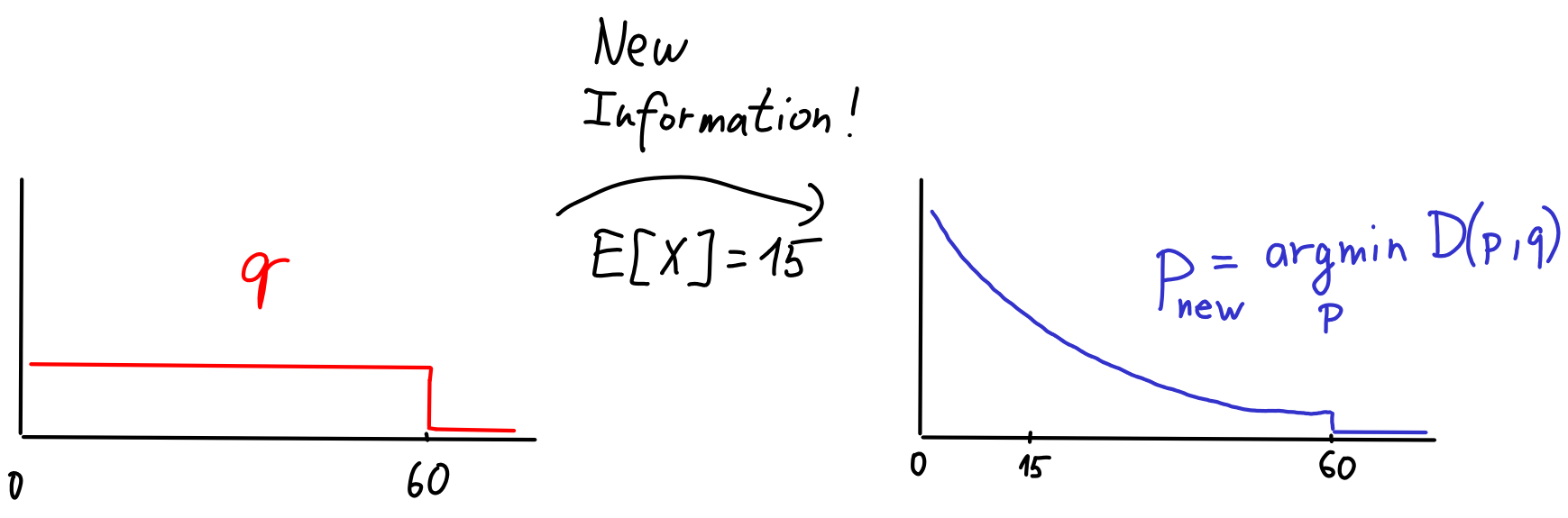
Let's try again. I eat many more lunches, but this time I keep recording the average time it takes me to eat lunch. Say, it turns out to be 15 minutes. How do I change $q$ to reflect this new information? The probability theory gives a clear answer.

We simply can't do this. In probability theory, we can condition on events like $X \le 30$, i.e., facts that are true for some values that $X$ can attain, but not others. But now we would like to condition on $E[X] = 15$ which is not an event, just a fact that's true for some distributions over $X$, but not others.

The fun part is that we can use KL divergence to 'condition' on $E[X] = 15$. It turns out that the most reasonable way to account for the new information is to choose as the model minimizing KL divergence to $q$. That is, for the set $P$ of distributions $p$ with $E_p[X] = 15$, choose

In the example, happens to look like exponential distribution:

This is sometimes called the minimum relative entropy principle. Why does this make sense? Intuitively, I want to find a distribution that would serve as the new best guess for what the truth is, while keeping the old model distribution as good a model of $p$ as possible. This is what we achieve by minimizing KL divergence $D(p, q)$.

Admittedly, this intuition may feel a bit shaky, as we typically prefer $p$ to represent the "true" distribution when using KL divergence, whereas here it's simply a new, improved, model. There's a more technical argument called Wallis derivation that explains why we can derive minimum relative entropy as "conditioning on steroids" from the first principles.

The maximum entropy principle

Let's delve deeper into the minimum relative entropy principle. One conceptual issue with it is that it only allows us to refine an existing model $q$ into a better model $p$. But how did we choose the initial model $q$ in the first place? It feels a bit like a chicken-and-egg dilemma.

Fortunately, there's usually a very natural choice for the simplest possible model $q$: the uniform distribution. This is the unique most 'even' distribution that assigns the same probability to every possible outcome. There's also a fancy name for using the uniform distribution as the safe-haven model in the absence of any relevant evidence: the principle of indifference.

It would be highly interesting to understand what happens when we combine both principles together. That is, say that we start with the uniform distribution (say it's uniform over the set $\{1, \dots, k\}$). What happens if we find a better model by minimizing KL divergence? Let's write it out:

I'm a one-trick pony—whenever I see KL divergence, I split it into cross-entropy and entropy:

In the previous chapter, it was the second term that was constant, now it's the first term: $\sum_{i = 1}^k p_i\log \frac{1}{1/k} = \log(k)$ does not depend on $p$, so minimizing KL divergence is equivalent to minimizing $-H(p)$. We get:

We've just derived what's known as the maximum entropy principle: given a set $P$ of distributions to choose from, we should opt for the $p\in P$ that maximizes the entropy $H(p)$.

General form of maximum entropy distributions

Let's now dive a bit deeper into maximum entropy. We'll try to understand what maximum entropy distributions actually look like. For example, we will see soon how does the maximum entropy distribution with $E[X] = 15$ looks like.

Here's what I want you to focus on, though. Let's not worry about concrete numbers like 15 too much. To get the most out of the max-entropy principle, we have to think about the questions a bit more abstractly, more like: If I fix the value of $E[X]$, what shape will the max-entropy distribution have?

For such a broad question, the answer turns out to be surprisingly straightforward! Before telling you the general answer, let's see a couple of examples.

If we consider distributions with a fixed expectation $E[X] = \mu$ (and the domain is non-negative real numbers), the maximum entropy distribution is the exponential distribution. This distribution has the form . Here, $\lambda$ is a parameter - fixing $E[X]$ to attain different values leads to different $\lambda$s. ¹

Another example: If we fix the values of both $E[X]$ and $E[X^2]$, the maximum entropy distribution is the normal distribution, where To keep things clean, we can rewrite its shape as for some parameters $\lambda_1, \lambda_2$ that have to be worked out from what values we fix $E[X]$ and $E[X^2]$ to.

Spot a pattern?

Note that this general recipe doesn't tell us the exact values of $\lambda_1, \dots, \lambda_m$. Those depend on the specific values of $\alpha_1, \dots, \alpha_m$, while the general shape remains the same regardless of the $\alpha$ values. But don't get too hung up on the $\alpha$s and $\lambda$s. The key takeaway is that the maximum entropy distribution looks like an exponential, with the "stuff we care about" in the exponent.

Catalogue of examples

Let's go through the list of maximum-entropy distributions you might have encountered. In fact, most distributions used in practice are maximum entropy distributions for some specific choice of functions $f_1, \dots f_m$.

So, when you come across a distribution, the right question isn't really "Is this a max entropy distribution?" It's more like, "For what parameters is this a max entropy distribution?" For example, you can forget the exact formula for the Gaussian distribution—it's enough to remember that using it implies you believe the mean and variance are the most important parameters to consider.

Let's go through the examples with this in mind. Please, do skip whatever doesn't ring a bell, the list is long.

Let's start with what happens if we don't have any constraints.

Logits, softmax, exponentials

If we believe the mean is an important parameter of a distribution (which is very typical), the max entropy principle states that the right family of distributions to work with are those with the shape:

This kind of distribution is known by many names, depending on its domain. Let's go through some instances!

Gaussians

If we fix both mean and variance, the max-entropy distribution is Gaussian.

We can now revisit our financial mathematics riddle from the intro.

Power-law

If you care about the scale of a random variable, maximum entropy leads to so-called power-law distributions.

And here's an application to our XKCD riddle:

Independence

One final example I find cute.

What's next?

In the next chapter, we'll see how the combo of maximum likelihood + maximum entropy explains the choice of loss functions used in machine learning.