Fisher information & statistics

In this chapter, we will explain a bit more about how KL divergence connects to statistics. In particular, one of the key statistical concepts is a so-called Fisher information, and we will see how one can derive it using KL divergence.

The polling problem

In one of our riddles, we have been talking about the problem with polling: If you want to learn the percentage of the vote for one party up to $\eps$, you need sample about $1/\eps^2$ voters.

The law of large numbers

One way to understand why we need $\Omega(1/\eps^2)$ samples is via the law of large numbers. This law tells you that if you flip a fair coin $n$ times, you typically get around $n/2 \pm O(\sqrt{n})$ heads. ¹. If your coin is biased and heads come out with probability $1/2 + \eps$, then the law says you will typically see around $(1+\eps)n/2 \pm O(\sqrt{n})$ heads. If you want to be able to separate the two options, you need the two intervals $n/2 \pm O(\sqrt{n})$ and $(1+\eps)n/2 \pm O(\sqrt{n})$ to be disjoint, which means that you have to choose $\eps$ such that $\eps \cdot n \approx \sqrt{n}$, i.e., $n$ should be at least around $1/\eps^2$.

KL intuition

But I want to offer a complementary intuition for the polling problem. Let's go all the way back to the first chapter where we introduced KL. Our running example was a Bayesian experimenter who wanted to distinguish whether his coin is fair or not fair. If the two distributions to distinguish are $(50\%, 50\%)$ and $(50\% + \eps, 50\% - \eps)$, then the problem of our experimenter gets extremely similar to the problem of estimating the mean up to $\eps$!

Remember, if we have two very similar distributions, KL between them is going to be positive, but very small. It turns out that

The intuition we should take from this is that each time we flip a coin, we get around "$2\eps^2$ bits of information" about whether the coin is fair or biased by $\eps$. Intuitively, once we get around 1 bit of information, we begin to be able to say which of the two coins we are looking at. We conclude that the number of trials we need to estimate the bias of a coin should scale like $n = 1/\eps^2$.

Fisher information

The trick with looking at KL divergence between two very similar distributions can be generalized further. Think of a setup where you have a family of distributions characterized by some number. For example:

• biased coins with heads-probability $p$ for all $p \in [0,1]$.
• gaussians $N(\mu, 1)$ for all $\mu \in \mathbb{R}$.
• gaussians $N(0, \sigma^2)$ for all $\sigma^2 \ge 0$.

More generally, think of a set of distributions $p_\theta$ parameterized by a number $\theta$.

One of the most basic tasks in statistics is that we have an empirical distribution $p$ and we want to find the $\theta$ so that $p_\theta$ fits the data the best, like below.

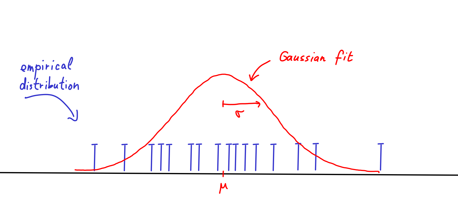
We have already seen this a few times, and we have seen in the chapter about minimizing KL why the maximum likelihood estimators are a reasonable approach to this.

But we can go a bit further -- if we assume that $p$ has literally been generated by one of the distributions $p_\theta$ for some $\theta$, we may ask how many samples we need to estimate $\theta$ up to additive $\eps$. Our polling question is just a special case of this more general question.

Our intuition about KL tells us if the data were generated by $p_\theta$, to estimate $\theta$ it's key to understand the value of . This is the general (and a bit opaque) formula we thus need to understand:

We will estimate the value of the right-hand side by computing the derivatives and . In particular, we will estimate with the following Taylor-polynomial approximation.

After plugging it in and some calculations ², we get

for

The term $I(\theta)$ is called Fisher information. Let's not try to understand what this integral mean. The short story is that you can approximate KL divergence of two similar distributions as $I(\theta)\cdot \eps^2$ and $I(\theta)$ can often be computed by integration.

Our KL intuition is telling us that estimating a parameter $\theta$ up to $\eps$ should require about many samples. Let's see what this intuition is saying in some cases:

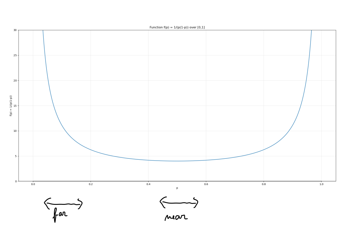
1. If you want to estimate $p$ of a biased coin, $I(p) = \frac{1}{p(1-p)}$. Thus, our KL intuition suggests that estimating the value of $p$ (with constant probability) should take about $p(1-p)/\eps^2$ samples. This is indeed the right formula (see the widget above).

2. If you want to find the mean of normal random variable with known variance $\sigma^2$, we have $I(\mu) = 1/\sigma^2$. Hence, our KL intuition suggests that estimating $\mu$ up to $\eps$ requires about $\sigma^2 / \eps^2$ samples.

3. If you want to find the variance of normal random variable with known mean $\mu$, we have $I(\sigma^2) = 1/(2\sigma^4)$. Hence, our KL intuition suggests that estimating $\sigma^2$ requires about $\sigma^4 / \eps^2$ samples.

In all above cases, it turns out to be the case that our intuition is correct and really describes how many samples you need to solve given problem. In fact, there are two important results in statistics: One of them is Cramér-Rao lower bound that basically says that our formula of $n = 1/(I(\theta)\eps^2)$ is indeed a lower bound. On the other hand, the so-called asymptotic normality theorem for MLE says that the MLE estimator is as good as our formula. ³

The upshot is that computing KL between two close distributions basically answers the most fundamental question of (frequentist) statistics -- how many samples do I need to get a good estimate of a parameter.

Fisher metric

Although KL divergence is asymetrical, it gets symmetrical in the limit. That is, if we do the computation for instead of , we would get the same expression up to some $O(\eps^3)$ terms. So, in this setup where we try to understand two distributions that are very close together, we can really think of it as being symetric. This way, we can define a proper distance function on the space of distributions -- it's called Fisher information metric and can give useful intuitions. For example, for the case of biased-coin-flipping distributions where coins have bias $p \in [0,1]$, we can represent all of them using a segment like this:

The Fisher information metric says that locally, the KL distance around a point $p$ is proportional to $I(p) = 1/(p(1-p))$. That is, the probabilities around $1/2$ are "closer together" than the probabilities at the edges. This is a supercharged-abstract-fancy way of saying what we have already seen many times -- probabilities should often be handled multiplicatively, not additively.